Automated data collection is fantastic, but..
Field-based research can be incredibly fun and rewarding - yet in many cases logistical challenges take the front seat when I think about my next outdoor stint. These challenges include site access, health and safety and training up personell as well as myself. But, first and foremost, I think about the data that I’ll be bringing back with me.
Ideally, I want to streamline and automate as much of the data collection and processing as possible, saving myself time, while ensuring reproducibility (added bonus! 😄). In an ideal world, all pertinent data would be collected by a set of loggers with a consistent output format, all resulting data files named applying a machine-readable scheme, and reading as well as processing the data could be automated (to a large extent).
But, alas, if you’ve done any type of field research, it’s likely you know that is often not the case. My latest encounter with such “troublesome” data presented an interesting challenge in terms of getting data into an analyses-ready format:
A set of Decagon EM50 loggers recorded soil moisture, soil tension and electrical conductivity in multiple locations, at various depths. I was getting tired of developing schemes/functions for each location, and decided to brainstorm for a ‘universal’ read_em50()! As so often recently, I thought: “tidyverse to the rescue!”
EM50’s and sensor types
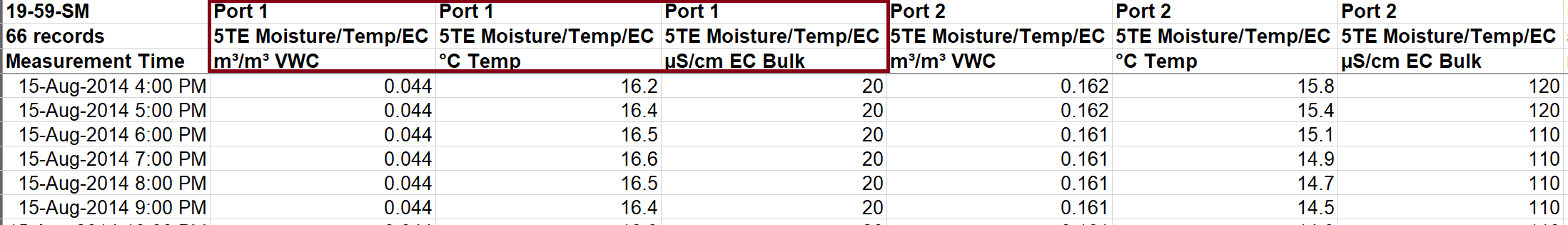
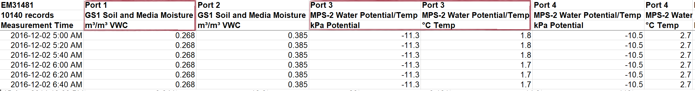
Decagon EM50 loggers can handle various sensor types in each port - a great advantage per-se. The output (i.e. table dimensions) depend on the sensors in operation and which variables they record. The examples below show that 5TE sensors provide three types of measurements, MPS-2 records two, and the GS1 provides one, for each connected port:
The tidy(verse) approach
My goal was to produce a “tidy” data set in long format, that can easily be queried - the three lines of meta data preceding the actual measurements are ideal for that, yet reading in the file in one go results in type issues (i.e. character vs. numeric). The real problem was that streamlining the read-in requires accounting for different set-ups (i.e. sensor types) at each location. After brainstorming a while, I came up with an approach that leveraged tidyr::gather(), tidyr::nest() and purrr::map() (a lot of the latter, in fact).
Briefly, in pseudo-code, the read_em50() function does the following, based on a directory containing EM50 output files:
- Read the first three lines of each file in the directory containing meta data
- Create one character string for each variable containing the port, sensor type and measurement unit.
- Read the remaining lines for each file in the directory containing the data
- Set the column names based on the strings in 2)
- Transform the data into long format (resulting in one time stamp, one measurement, and one “meta string” column)
- Nest the data, and subsequently use the “meta string” to generate individual columns for ports, sensor type and measurement units.
The function
read_em50() ended up relying heavily on the series of map functions from purrr. I’ve slowly but surely shifted toward using map() (and the likes of) to do most of my ‘batch processing’, as I very much appreciate the consistent syntax. Here it is:
#' Read EM50 files from a directory in batch
#'
#' @description This function allows reading an entire directory of EM50 logger files. Files within one directory should have a consistent pattern (i.e. sensor set-up), reflecting one logger / location.
#' @param fpath Character string. Path to the directory containing EM50 files.
#' @param site_id Character string. Unique identifier for each site, corresponding to the _fpath_ directory
#'
#' @return A list, with individual tibbles for each directory/site, containing key meta and identifier columns, and a nested data column of time stamps and corresponding measurements.
#' @export

read_em50 <- function(fpath, site_id){
        require(readxl)
        require(purrr)
        require(dplyr)

        fnames <- list.files(fpath, full.names = TRUE, pattern = "*.xls*")

        # extract meta information (first three lines) for all files
        meta <- map(fnames,
                    readxl::read_excel,
                      n_max = 3,
                    col_names = FALSE) %>%
                # create one meta string for all info in one column
                map(~apply(.x, MARGIN = 2, paste0, collapse = "_")
                             ) %>%
                # rename date time column
                modify_depth(1,
                             ~modify_at(.x,
                                        1,
                                        function(x) stringr::str_replace(x, ".*", "date_time")
                                        )
                             ) %>%
                map(as.character)


        # drop columns in original file resulting from ports missing sensors
        if(any(map(meta, ~any(grepl("None", .x))))){

                keep_cols <- map(meta, ~!grepl("None", .x)) %>%
                        map(~which(.x == TRUE))

                meta <- map2(meta, keep_cols, ~`[`(.x,.y))
        }


        # read in all data as numeric (results in numeric excel dates)
        temp_data  <- map(fnames,
                          readxl::read_excel,
                          skip = 3,
                          col_names = FALSE,
                          col_types = "numeric") %>%
                # use meta string to set column names
                map2(meta, ~set_names(.x, .y)) %>%
                # account for numeric dates
                map(~mutate(.x,
                            date_time = as.POSIXct("1899-12-30", tz = "MST") +
                                    date_time * 3600 * 24 )) %>%
                # make data long
                map(~tidyr::gather(.x, -date_time, key = "col_names", value = "value")) %>%
                bind_rows() %>%
                dplyr::distinct() %>%
                tidyr::nest(-col_names) %>%
                # use meta column to produce additional columns for port, sensor and measurement
                mutate(port = stringr::str_extract(col_names, "Port [:digit:](?=_)"),
                       sensor = stringr::str_extract(col_names, "(?<=_).*(?=_)"),
                       # unit = stringr::str_extract(col_names, "([^_]*)[^ ]$")
                       # %>% stringr::str_extract(".*(?<= )"),
                       measure = stringr::str_extract(col_names, "([^ ]*)$"),
                       site = site_id,
                       col_names = NULL)


        return(temp_data)


}
In action, it then looks as follows:
library(purrr)
library(tidyr)
library(dplyr)

# set file paths
fpaths <- list.dirs("./2018-11-24-tidy-em50/dat",
                    full.names = TRUE,
                    recursive = FALSE)

# extract site locations from directory names
site_ids <- gsub(".*/", "", fpaths)

# run the function!
em_data <- map2(fpaths,site_ids,
                ~read_em50(fpath = .x,
                  site_id = .y))


# read_em50 produces a list of tibbles, one for each directory/site
# this step simply produces the final tibble
em_data_flat <- em_data %>%
        bind_rows()


# replaced the nested tibble with a char. string for easier viz
knitr::kable(x = em_data_flat %>%
                   mutate(data = "nested df") %>%
                   head(5),
             format = "html",
             caption = "A quick look at the first five rows of the resulting tibble.
Note, the actual nested tibble was replaced with a character string for visualization.")| data | port | sensor | measure | site |
|---|---|---|---|---|
| nested df | Port 1 | 5TE Moisture/Temp/EC | VWC | 19-59 |
| nested df | Port 1 | 5TE Moisture/Temp/EC | Temp | 19-59 |
| nested df | Port 1 | 5TE Moisture/Temp/EC | Bulk | 19-59 |
| nested df | Port 2 | 5TE Moisture/Temp/EC | VWC | 19-59 |
| nested df | Port 2 | 5TE Moisture/Temp/EC | Temp | 19-59 |
Unfortunately, my regex skills are sub-par, and I was only able to capture part of the measurement unit. Any help / comments would be greatly appreciated if you end up applying this function.
Adding additional info/meta data (e.g. sensor depths, soil characteristics) from another source (e.g. *.csv) is then simply done with a table join:
library(tidyr)

sensor_meta <- read.csv("./2018-11-24-tidy-em50/dat/meta.csv",
                        stringsAsFactors = FALSE)

em_data_flat_join <- em_data_flat %>%
        left_join(sensor_meta,
                  by = c("site", "port"))
# replaced the nested tibble with a char. string for easier viz
knitr::kable(x = em_data_flat_join %>%
                   mutate(data = "nested df") %>%
                   head(5),
             format = "html",
caption = "First five rows of the data in its final output format")| data | port | sensor | measure | site | project | pond | depth_m |
|---|---|---|---|---|---|---|---|
| nested df | Port 1 | 5TE Moisture/Temp/EC | VWC | 19-59 | URSA | 19 | 0.10 |
| nested df | Port 1 | 5TE Moisture/Temp/EC | Temp | 19-59 | URSA | 19 | 0.10 |
| nested df | Port 1 | 5TE Moisture/Temp/EC | Bulk | 19-59 | URSA | 19 | 0.10 |
| nested df | Port 2 | 5TE Moisture/Temp/EC | VWC | 19-59 | URSA | 19 | 0.25 |
| nested df | Port 2 | 5TE Moisture/Temp/EC | Temp | 19-59 | URSA | 19 | 0.25 |
library(ggplot2)

em_data_flat_join %>%
      filter(site == "19-59") %>%
      tidyr::unnest() %>%
      ggplot(aes(x = date_time,
                 y = value,
                 color = as.factor(depth_m))) +
      geom_line() +
      labs(x = "Date",
           y = "Value",
           title = "Soil electrical conductivity, temperature and vol. water content for Site 19-59",
           color = "Depth (m)") +
      facet_grid(measure~.,
                 scales = "free_y") +
      theme_bw()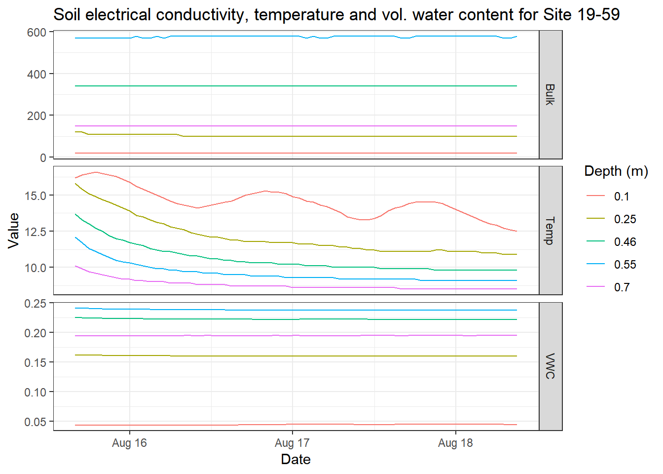
Wrapping up
The function has proven extremely helpful for pulling together data of interest quickly, as well as in producing exploratory and subsequent, higher-quality visualizations. Next to the saved time, what I ejoyed most was brainstorming and finding the simplest “one size fits all” approach. Yet, the function seems to be fairly slow, as there is quite a bit of copying around involved with carrying over the meta character string. A few improvements that I may implement in the future include 1) parallelization for a speed boost, 2) making the column renaming more efficient, and 3) providing more optional arguments to read_em50() that allow pre-defining ports / sensor types for the read-in process. I’d also very much appreciate any feedback and suggestions on improving my use of map() - or limiting it by providing alternatives.