A basic operation
Joining tables by a common key is frequently required by anybody working with data (and especially relational databases) - and an approach that isn’t too difficult to master luckily! This post will showcase how simple and rolling joins work in data.table (and also documents my learning process with this wonderful package). I’ve fallen in love with the latter (rolls) for setting up model grids, which I will demonstrate.
The tidy dplyr way
Typically I’ve used the join family of functions from dplyr:
inner_join()left_join()right_join()full_join()semi_join()nest_join()anti_join()
These work fabulously in pipes and have a consistent, and tidyversesque (🤓) API. These functions are part of my basic, data wrangling, munging and handling tool set, and come in very handy when matching up e.g. different measurements for similar sites and/or dates!
Example
library(dplyr)

# create a dummy data frame with data
temperatures <- expand.grid(area = c("east", "west"),
                     site = letters[1:3]) %>%
      mutate(temp_c = runif(n = nrow(.), -5, 5))

# create a table related via common key 'site'
vegetation <- data.frame(site = letters[1:3],
                          landcover = c("forest",
                                        "steppe",
                                        "wetland"),
                         stringsAsFactors = TRUE)


# magic!
overview <- left_join(temperatures, vegetation, by = "site")

knitr::kable(overview,
             format = "html",
             digits = 1,
caption = "Joined data set.")| area | site | temp_c | landcover |
|---|---|---|---|
| east | a | 3.8 | forest |
| west | a | -3.6 | forest |
| east | b | 4.4 | steppe |
| west | b | 2.1 | steppe |
| east | c | 3.3 | wetland |
| west | c | 4.9 | wetland |
Aggregation is just two lines away:
overview_summary <- overview %>%
      group_by(landcover) %>%
summarise_if(is.numeric, mean)| landcover | temp_c |
|---|---|
| forest | 0.1 |
| steppe | 3.2 |
| wetland | 4.1 |
Setting the data.table
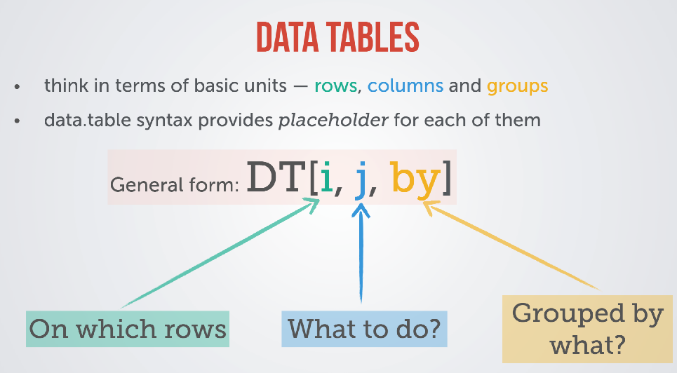
In short, data.table is an incredibly powerful and resource-efficient package, that I just began using and loving. It’s syntax is initially a bit difficult to wrap your head around - but that holds true for pretty much any new API/package I started using. It has outstanding documentation (e.g. this intro vignette) and is well-maintained. And so much fun!
This here is taken straight from the introductory PDF, and says it all:
Example
I’ll use the same example data from above to show a few data.table tricks. data.tables require keys to operate on and need to be set manually, or through coercion using as.data.table().
library(data.table)

# create a dummy data frame with data
temperatures <- expand.grid(area = c("east", "west"),
                     site = letters[1:3]) %>%
      mutate(temp_c = runif(n = nrow(.), -5, 5)) %>%
      as.data.table()

# create a table related via common key 'site'
vegetation <- data.table(site = letters[1:3],
                          landcover = c("forest",
                                        "steppe",
                                        "wetland"),
                         stringsAsFactors = TRUE)


# magic!
# overview_dt <- DT

temperatures[vegetation, on = "site"]
## area site temp_c landcover
## 1: east a -2.781943 forest
## 2: west a 3.062782 forest
## 3: east b -4.427340 steppe
## 4: west b -4.528919 steppe
## 5: east c 0.690448 wetland
## 6: west c -4.127972 wetland# or after setting keys specifically
setkey(temperatures, site)
setkey(vegetation, site)
overview_dt <- temperatures[vegetation]| area | site | temp_c | landcover |
|---|---|---|---|
| east | a | -2.8 | forest |
| west | a | 3.1 | forest |
| east | b | -4.4 | steppe |
| west | b | -4.5 | steppe |
| east | c | 0.7 | wetland |
| west | c | -4.1 | wetland |
And as above, a simple aggregation, yet on a single line:
# same aggregation as before:
overview_dt_summary <- overview_dt[,j = .(temp_c_mean = mean(temp_c)), by = .(landcover)]| landcover | temp_c_mean |
|---|---|
| forest | 0.1 |
| steppe | -4.5 |
| wetland | -1.7 |
Note how we always come back to the simple syntax of DT[i, j, by] (where, what, grouping). (Side note: the .() syntax indicates that the input type is a list, important when you want to return a named column or use multiple columns to operate on).
All operations, for example, can be done on subsets of the data, too, and multiple calculations in one go are very much possible.
overview_dt[area == "east", j = .(count = .N, max_temp_c = max(temp_c))]## count max_temp_c
## 1: 3 0.690448Getting fancy with a (simple!) rolling join
The problem
The main reason I stumbled over data.table were rolling joins. I was desperately looking for a convenient way of assigning parameters to a 1-D model grid. More precisely, I was simulating lateral flow through a soil column, and wanted to be able to set the stratification in a consistent manner that was independent of my choice of discretization (i.e. how thick each simulated slice of the soil column would be).
There are a few ways I thought this could be achieved by (and certainly more than I could come up with). My starting point was always a table containing general parameters, the soil profile, and a model grid that needs to be populated with the profile based on the general parameters. My ideas were:
- looping over each row in the model grid and filling a “soil_type” column based on a conditional statement
- using
dplyr::mutate()with a nestedifelse() - using a
dplyr::case_when()with conditional statements covering the extent of each soil layer - hard-coding a base
Rsolution with[]subsetting and conditional statements
While all of these are pretty-straight forward, I was hoping for something that could be employed in a more programmatic fashion. Enter data.table
Conditional joining with DT[ , roll = TRUE/-Inf]
A rolling join matches one row of a table with that of another (based on a common key), as long as the matching condition has not changed. A quick demonstration!
times <- data.table(hour_of_day = 1:24)
mood <- data.table(hour_of_day = c(0, 8, 20, 24),
                   feeling = c("sleep", "coffee please", "ready for bed", "sleep"))

# regular join
mood[times, on = "hour_of_day"]
## hour_of_day feeling
## 1: 1 <NA>
## 2: 2 <NA>
## 3: 3 <NA>
## 4: 4 <NA>
## 5: 5 <NA>
## 6: 6 <NA>
## 7: 7 <NA>
## 8: 8 coffee please
## 9: 9 <NA>
## 10: 10 <NA>
## 11: 11 <NA>
## 12: 12 <NA>
## 13: 13 <NA>
## 14: 14 <NA>
## 15: 15 <NA>
## 16: 16 <NA>
## 17: 17 <NA>
## 18: 18 <NA>
## 19: 19 <NA>
## 20: 20 ready for bed
## 21: 21 <NA>
## 22: 22 <NA>
## 23: 23 <NA>
## 24: 24 sleep
## hour_of_day feeling# forward join populates until a condition changes (i.e. a new match in the "on" column is found)
mood[times, on = "hour_of_day", roll = TRUE]## hour_of_day feeling
## 1: 1 sleep
## 2: 2 sleep
## 3: 3 sleep
## 4: 4 sleep
## 5: 5 sleep
## 6: 6 sleep
## 7: 7 sleep
## 8: 8 coffee please
## 9: 9 coffee please
## 10: 10 coffee please
## 11: 11 coffee please
## 12: 12 coffee please
## 13: 13 coffee please
## 14: 14 coffee please
## 15: 15 coffee please
## 16: 16 coffee please
## 17: 17 coffee please
## 18: 18 coffee please
## 19: 19 coffee please
## 20: 20 ready for bed
## 21: 21 ready for bed
## 22: 22 ready for bed
## 23: 23 ready for bed
## 24: 24 sleep
## hour_of_day feeling# backwards works, too!
mood[times, on = "hour_of_day", roll = -Inf]## hour_of_day feeling
## 1: 1 coffee please
## 2: 2 coffee please
## 3: 3 coffee please
## 4: 4 coffee please
## 5: 5 coffee please
## 6: 6 coffee please
## 7: 7 coffee please
## 8: 8 coffee please
## 9: 9 ready for bed
## 10: 10 ready for bed
## 11: 11 ready for bed
## 12: 12 ready for bed
## 13: 13 ready for bed
## 14: 14 ready for bed
## 15: 15 ready for bed
## 16: 16 ready for bed
## 17: 17 ready for bed
## 18: 18 ready for bed
## 19: 19 ready for bed
## 20: 20 ready for bed
## 21: 21 sleep
## 22: 22 sleep
## 23: 23 sleep
## 24: 24 sleep
## hour_of_day feelingDiscretizing a soil profile for a simple model
As noted earlier, I stumbled over data.table while looking for the most convenient way of assigning soil properties to cells along a soil profile in a programmatic fashion. This was principally necessary for a simple sensitivity analyses checking the impact of my model discretization, i.e. thickness of each cell / slice along the soil profile from surface to the model boundary (e.g. bedrock).
I used a list to store all of the basic model parameters in model_params:
- total depth of soil column (\(z\))
- height of each cell (i.e. \(\Delta z\))
The number of cells is then derived as \(n = \frac{ z } {\Delta z}\).
Additionally, I pulled soil profile and texture data from a soil coring log of our field sites and stored them in soil_param as a data frame. The data shown here are a simplified ‘dummy’ set.
model_params <- list(total_depth = 0.8,
                     cell_height_m = 0.1)
# model_params$n_cells = model_params$total_depth / model_params$cell_height_m

# starts from bottom
soil_params <- data.table(z = c(0.4, 0.1, 0),
                         soil_type = c("silt", "organic_mineral_mix", "lfh"),
                         ksat = c(10^-8, 10^-5, 10^-4),
                         key = "z")
I then developed a simple function model_domain() that used a rolling join and returned a data.frame with an option to set total depth and cell height.
#' Creates a discretized model domain along a soil profile
#'
#' @param total.depth Depth of soil column in meters
#' @param cell.height Height of each model cell in meters
#' @param soil.params A data frame containing one column of soil depths (named 'z')and any number of additional parameters of interest. These are added to the model grid using a rolling join. These parameters must be supplied ordered from top to bottom, starting at the respective depths, with zero (0) denoting the soil surface.
#'
#' @return Returns a data frame representing a soil column and has at least one column for soil depths, discretized based on the supplied cell.height
#' @export
#'
#' @examples
model_domain <- function(total.depth, cell.height, soil.params){
      require(data.table)

      soil.params <- data.table(soil.params, key = "z")

      domain <- data.table(z = seq(0, total.depth, by = cell.height), key = "z")


      joined <- soil.params[domain, on = "z", roll = TRUE]


      return(joined)

}
Giving it a spin:
profile_0.1 <- model_domain(total.depth = model_params$total_depth,
             cell.height = model_params$cell_height_m,
             soil.params = soil_params)

profile_0.1
## z soil_type ksat
## 1: 0.0 lfh 1e-04
## 2: 0.1 organic_mineral_mix 1e-05
## 3: 0.2 organic_mineral_mix 1e-05
## 4: 0.3 organic_mineral_mix 1e-05
## 5: 0.4 silt 1e-08
## 6: 0.5 silt 1e-08
## 7: 0.6 silt 1e-08
## 8: 0.7 silt 1e-08
## 9: 0.8 silt 1e-08Now, the model_domain() function can be easily used to investigate the impact of varying parameters of the model, and corresponding soil horizons. Rather than a formal investigation, here I’ll only offer a visual representation of how different \(\Delta z\)’s affect the model domain.
library(dplyr)
library(ggplot2)

# make a series of cell heights to discretize the model with
model_params$cell_height_m <- seq(0.02, 0.1, by = 0.02)


# use map (apply-style function) to run model_domain with multiple cell heights
profile_multiple <- purrr::map(model_params$cell_height_m,
                               ~model_domain(total.depth = model_params$total_depth,
                                             cell.height = .x,
                                             soil.params = soil_params)) %>%
      # supply names for subsequent binding and plotting
      purrr::set_names(model_params$cell_height_m) %>%
      bind_rows(.id = "height")


# make plot
profile_multiple %>%
      ggplot(aes(x = "Profile",
                 y = z,
                 fill = soil_type)) +

      # add points
      geom_point(size = 3,
                 shape = 21,
                 color = "gray50") +

      # split for each Delta z
      facet_grid(~height,switch = "x") +

      # labelling
      labs(y = "Depth",
           fill = "Horizon",
           title = "Model Domain with variable Discretization",
           subtitle = "Resolution impacts location of boundaries" ) +

      # scales
      scale_y_reverse() +
      scale_fill_viridis_d(begin = 0, end = 0.9,option = "D") +

      # theming
      theme_minimal() +
      theme(plot.background = element_rect(fill = "transparent"),
            panel.border = element_rect(fill = NA, color = "transparent"),
            text = element_text(color = "gray40", face = "italic"),
            axis.title.x = element_blank(),
            axis.text.x = element_blank())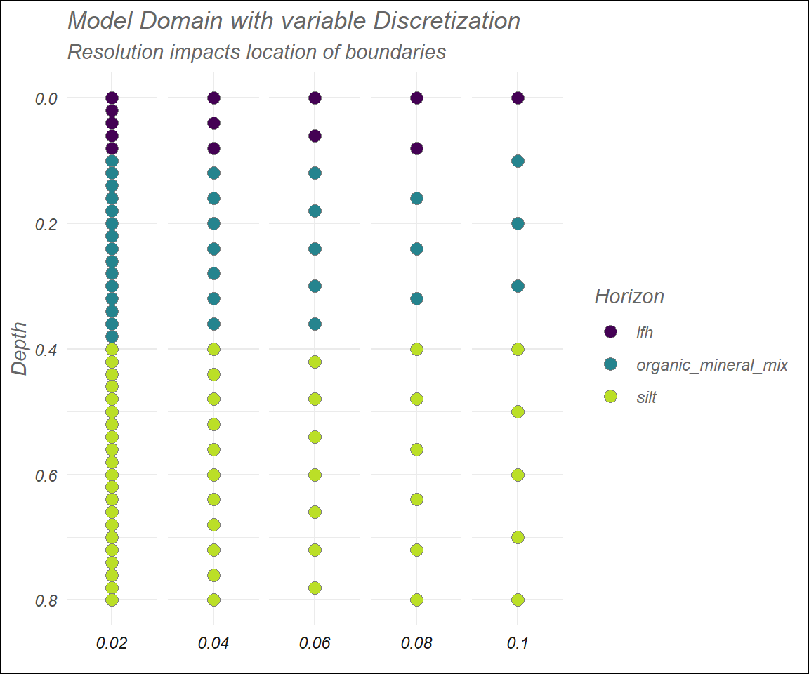
data.table is a new favorite!
I hope that you, just like me, have found a new friend in the #rstats world with data.table. The use-case I showed here was fairly basic, yet it can be applied in a number of settings, and I’ve found it particularly useful for making model grids. Yet, I can see a number of other applications, such as matching pre-defined or computed events, such as droughts, storms or disturbances between time series of interest. Give it a go yourself, and let me know which applications you can think up.